Difference between revisions of "Category:Standard diagram"
(Created page with "Category:Diagrams ===Standard diagram=== You will get to use the spread sheet editor whenever you want to edit a standard diagram. Standard diagrams are typically added...") |
(No difference)
|
Revision as of 05:35, 29 March 2011
Standard diagram
You will get to use the spread sheet editor whenever you want to edit a standard diagram. Standard diagrams are typically added directly in document and presentation editors. You can also set up standard diagrams from the diagram resource list.
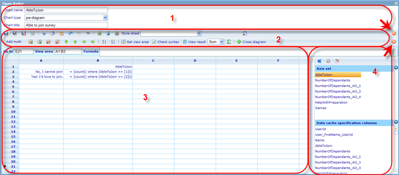
Since the spread sheet editor works the same both of these places we will describe it all here. Please look below to see how the spread sheet editor looks!
The spread sheet area consists of 4 main areas;
1: The name and diagram specification area
2: The action button area
3: The expression sheet area
4: The data source area
We will explain each of these areas in turn below. We will start by describing area 3 and 4, since these form the basic understanding of what we use area 1 and 2 for.
The expression sheet area
Most users will feel quite comfortable using the expression sheet, since it is very similar to other spread sheet software. Generally we specify labels in the first column and row of the sheet and then the data in the cells that stand between the coordinates of the rows and column headers. To navigate in this area you can use the arrow buttons of your key board. To type into a cell and replace anything that was in the cell before, just start typing while the cell is highlighted. If you want to edit the content of a cell you must double click on it with your left mouse button. To exit from a cell you can use the return button.
It is possible to highlight larger areas at the same time, e.g. by clicking a row-cell in the column on the far right of the sheet, you will highlight an entire row:
A similar action can be done to highlight a column, clicking on the column header.
Finally you can highlight a specific area in the sheet by left clicking with your mouse on a cell and while holding the button down, moving your mouse to another cell in the sheet and letting go. This will highlight all cells in the area between the initial and final cell. Below is an example!
When you have highlighted one or multiple cells in the spreadsheet there are a lot of buttons that you can use from the action button area to affect these cells.
If you cannot see the full content of a cell you can change the column width by dragging the border between columns to the right. You can also highlight any cell and the content of that cell will be visible and editable in the 'Formula' area on top of the expression area.
The 'View area' indicates which area of the expression sheet would be used for a diagram in case you choose to save your work at this very moment. We will later explain to you how you can change the view area to your liking!
The 'Go to' field always shows you your current highlighted position in the expression sheet. You can update directly in this field to move the highlighted area.
In the cells above you will see that 'expressions' exist instead of 'numbers' in the cells B2 and B3. These expressions will, if 'calculated', contact a data cache to convert the expression to an actual number. Users making spread sheets can choose to use expressions to represent numbers or actually just write numbers directly into a cell. The spread sheet will know whether the content of a cell is representing an actual value or an expression that needs conversion, simply by whether or not the content of the cell starts with the symbol '='. To learn more on making expressions please click here.
The data source area
Notice that there is a red horizontal arrow button on the far left of the action area. This button is used to show/hide the data source area.
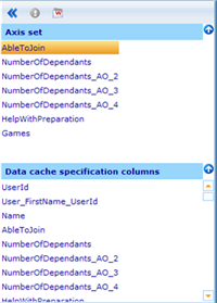
The data source area will be empty of no data cache is chosen for the spread sheet. There are two ways in which data may exist. If the spread sheet is added as a diagram from inside a report template, then the spread sheet will automatically presume it should use the same data cache as the template. If the template does not have a data cache or the spread sheet is not created from within a template, the user must specify the data cache using the applicable button in the action area of the spread sheet. Once we have managed to have a data cache related to the spread sheet the area may look something like below.
The data area consist of two separate lists that both have something to do with the chosen data cache. The axis set list holds information on possible answer options to a data column and mathematical information like what is to be used as base for an axis. The axis set lets us set up quite extensive logics for how to represent data in a diagram and to understand this in depth please refer to the help files on this by clicking here! The data cache specification columns define the actual names that can be used as variables in expressions. To learn more about the structure of data cache specifications please click here!
There are two important buttons in the tool bar of the data source area; the double arrow button and the information button.
The double arrow button![]() is active both when highlighting a row in the axis set and data cache lists. If user clicks this button with an axis set row highlighted, it will generate the entire structure needed for a diagram using the chosen axis. Please be aware that this will remove any values that was already inserted into the expression sheet area. If using the button with a data cache column highlighted, it will instead just insert the column name into the position the user is in the spread sheet.
is active both when highlighting a row in the axis set and data cache lists. If user clicks this button with an axis set row highlighted, it will generate the entire structure needed for a diagram using the chosen axis. Please be aware that this will remove any values that was already inserted into the expression sheet area. If using the button with a data cache column highlighted, it will instead just insert the column name into the position the user is in the spread sheet.
The information button ![]() is only available when a data cache column is highlighted. This will open a small dialog giving some background information of the question the column was initially derived from and information like type and answer options.
is only available when a data cache column is highlighted. This will open a small dialog giving some background information of the question the column was initially derived from and information like type and answer options.
The name and diagram specification area
The diagram area will show three different fields most of the time. If user chooses 'Table diagram' as chart type, there will be some additional information required for subtitles of the table.
These are the values user must set:
Name: Give your spread sheet a unique and recognizable name!
Chart type: Depending on the chart type you choose there will be restrictions to what you can set the view area as! When choosing 'Table diagram' there will further be a couple of additional fields into which information can be added.
- Pie diagrams can only have one series, but as many items as wanted. The view area must therefore have exactly two columns. One column is the labels and the other is the results.
- Table diagrams have no view area limitations. When choosing table diagrams you will be offered to supply two additional pieces of information; namely sub title 1 and 2.
- Point charts can have as many series as the user wants, but only two data values for each. The view are must therefore have exactly three rows. Row 1 specifies the label of a point in the chart and the next two rows the x and y coordinates.
- Radar, area and bar-line charts have no restrictions on number of rows and columns.
Chart title: This is used for pie, point, radar, area and bar-line charts. It places a title inside the chart image being created.
Sub title 1: Will place a title in the top left area of the table that specifies what the records in the x-axis illustrate.
Sub title 2: Will place a title over columns 2 and higher that explain what the columns of the y-axis show.
The action button area
The action bar works together with the entire spread sheet and in particular with the expression sheet area to configure the final data and diagram. Below is an illustration of the action bar and numbers to identify each one.
1- Save buttons: The save buttons you have available will differ slightly depending on where you are editing the spread sheet from. Common save methods are 'Save' and 'Save and close'. When editing from inside a template you will also have a 'Save and next', which will immediately bring you to the next spread sheet diagram in the template. This is a quick way to move between diagrams. When in a spread sheet in the resource spread sheet list you will also have a 'Save as' button, which will make it possible to save a new copy of the spread sheet you are working on under a different name than the one you initially opened!
2 - Preview diagram: Clicking this button will make it possible for you to preview the diagram of the spread sheet. This is a good way to check whether styles and date work and look good together.
3 - Cut, copy and paste: You can highlight part of strings, cells, columns, rows or areas and copy/cut and paste them to different locations. You can also use short cuts for cut (ctrl-x), copy (ctrl-c) and paste (ctrl-v) to perform these actions.
4 - Undo - redo: If you made a mistake you can use the undo button to regret the action and move back a step. If you undo something that you found out you do not want to undo anyway, you can click the redo button to go one step forward.
5 - Find and replace: You can choose the area in which you want to 'Find' by highlighting the relevant area of cells. Adding a text to the 'Find what' field you can then click 'Find' to have shown one result at a time or 'Find all' to have all shown in one go. If you only wish to return result that Match cases exactly or where the Find what string matches a cell completely, then you can click these search filters in the dialogue. If you wish to replace the found results with another text you should put this text in the 'Replace with' field and user the replace buttons.
6 - Export to excel: Will export all the contents of your expression sheet area to an excel sheet. If viewing the table as results then the results will be exported. If viewing as expressions then the expressions will be exported.
7 - Data cache specification: To add a data cache to your diagram you can click this button. If you are working from a template the diagram might already be inheriting its data cache from this. It is although possible to overwrite the template data cache in connection with this diagram by specifying another data cache here. To learn more on data cache specifications, please click here.
8 - Set inline styles: By using this button we will open a dialog where we can set inline styles for the diagram. To learn more about diagram styling and inline styles, please click here.
9 - Attach a style sheet to the spread sheet diagram: Shows a drop down list of all style sheets in the system. This is a level higher than spread sheets given via inline styles. To understand style sheets and the levels at which they can be assigned, please click here!
10 - Change diagram: This drop down is only available when we are editing diagrams inside templates. Instead of having to save and close the spreadsheet editor and the find the diagram we want to modify afterwards in the template editor, we can simply move between diagrams using this drop down.
11 - Close: Close button for the spread sheet editor.
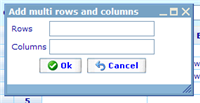
12 - Add multi: Since the spread sheet is made in a browser we cannot support an endless number of rows and columns in the direct view area as similar desktop applications can. When you want to expand the area in which you are building your spread sheet you can use this button to add multiple extra columns and rows to the view area at once.
13 - Add/remove rows/columns: When standing on a cell or area you can click the add buttons and an extra column/row will be added next to your highlighted area. By highlighting one or more cells, columns or rows you can also ensure that all rows/columns in this area are deleted by clicking the remove buttons.
14 - Move rows/columns: By highlighting cells, rows, or columns and using these arrows you can swap contents of entire rows or columns. If you highlight a cell in column B and click the left direction arrow, the all the content of column A will B moved to column B and visa versa.
15 - Sort: Highlight a column and sort that column. If data exists in other columns action will require you to answer if you want to expand the selection being sorted.
16 - Set view area: Specifies which cells will be used for the diagram you are making. This makes it possible to have intermediary calculations outside the shown diagram, which are used as part of a calculation inside the diagram.
17 - Check syntax: This feature checks if you have made any illegal syntax in the expression sheet area. Any expression seen as illegal will be shown in red font after checking is finished.
18 - View result: Clicking this button will make an immediate calculation of all expressions in your spread sheet and show the results directly in the expression sheet area. To return to the expression view mode just click on any cell! Notice that the calculations done with this button does not take into account any constants or filters defined at the report level!
19 - Generate result cells: By highlighting a number of cells and clicking the 'S' symbol you will insert a cell at the bottom with the expression type stated in the drop down to the left of that symbol. By changing the value in the drop down the inserted expression will also change next time you use the 'S' button.
20 - Cross diagram: This will open a limited version of the cross diagram viewer, making it possible for you to create the expression in a much simpler manner that writing each one individually.To understand the cross diagram editor better, please click here!
21 - Constants: To insert constants into any expression, just find it using this dialog. To understand the use of constants please click here!
Pages in category "Standard diagram"
This category contains only the following page.


